Computer Vision Tutorial Series: Part 1 — Intro to Computer Vision

9 min readJun 29, 2024

PS. I will provide the codes based on colab notebook so that we may need some colab-specific packages/libraries from time to time. But if you work in a local or different environment, you can ignore them.
PS. These tutorials are initially prepared for Computer Vision course at Sabanci University. Therefore I didn’t plan on sharing these tutorials when I was preparing them. For this reason, some of them don’t have references. However, if you notice any references, please let me know so I can add them :)
Finally, you can find the related codes in this notebook.

Setup

First, we need to install and import some libraries.

!pip install opencv-python                   # install opencv

import cv2                                   # for image operations
import matplotlib.pyplot as plt              # for visualisation
import numpy as np                           # for numerical operations
from google.colab.patches import cv2_imshow  # for displaying images on colab

Basic Operations with OpenCV

Reading an Image

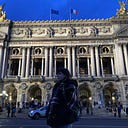
img_path = f"{image_folder}/opencv_intro1.jpg"     # the path to the image

img_color = cv2.imread(img_path)                   # reading the image

Color images have multiple color channels; each color image can be represented in different color models (e.g., RGB, LAB, HSV).

Image is a numpy array of shape (height, width, channels). So if we print our image, we will see something like this:

print(image)

>>> array([[[ 18,  65, 126],
           [ 17,  64, 125],
           [ 17,  64, 125],
           ...,
           [ 67, 143, 219],
           [ 61, 139, 216],
           [ 59, 136, 215]],
           ...,
           [ 35,  57,  93],
           [ 27,  49,  85],
           [ 22,  44,  80]]], dtype=uint8)

And if we use .shape to see it’s shape:

print(img_color.shape)   # (height, width, channels)

>>> (253, 430, 3)

Displaying an Image

cv2.imshow() function opens a window and displays the specified image in it. The window remains open until the user presses any key. After the user presses a key, the window closes. It takes two arguments: the title of the window and the image to be displayed.
In colab we can use cv2_imshow() instead of cv2.imshow() since colab does not support popup windows.

cv2_imshow(img_color)

**sample output for** cv2_imshow(img_color)

Displaying an Image using Matplotlib

We can also use matplotlib library to display images. We will use previously imported matplotlib.pyplot at this point:

plt.imshow(img_color)

**sample output for** plt.imshow(img_color)

Note that; matplotlib reads a color image in RGB (Red, Green, Blue) manner only, but OpenCV reads the color image in BGR (Blue, Green, Red) format. So, if we will use matplotlib for visualisation purposes, we need to convert our image’s color mode:

# convert BGR to RGB while displaying the image using matplotlib
# reverse the order of elements along the last axis

plt.imshow(img_color[: , : , ::-1])

**sample output for** plt.imshow(img_color[: , : , ::-1])

Reading and Displaying a Grayscale Image

Grayscale Images have a wider range of intensity than black and white. Each pixel is a shade of gray with pixel values ranging between `0` (black) and `255` (white).

To read the image in grayscale we need to specify a flag that specifies the way how the image should be read:

img_gray = cv2.imread(img_path, cv2.IMREAD_GRAYSCALE)    
cv2_imshow(img_gray)

PS. Instead of using cv2.IMREAD_GRAYSCALE we can also use 0 to read the image in grayscale.

This time, our image is a numpy array of shape (height, width). And if we print its shape we will see something like this:

print(image.shape)

>>> (253, 430)

Accessing & Changing Pixel Values of an Image

We can use indexing like we use for lists to access a pixel of an image. For ex. accessing the pixel at (100, 150) of the image (100th row, 150th column) would look like this:

img_gray[100, 150]

Again, we can use indexing to access a range of pixels. Accessing the pixels from (100, 200) to (120, 210) in the image → (100th row to 120th row, 200th column to 210th column):

img_gray[100:120, 200:210]

To change the pixel values of an image, we can select a range via indexing and set the range to a value. For ex. let’s select a range and set it to white:

img_color[100:120, 200:400] = (255, 255, 255) # setting the pixel value
cv2_imshow(img_color)

Saving an Image

To save an image, we can use cv2.imwrite(). We just need to specify the path where we want to save it:

cv2.imwrite("saved_image.jpg", img_color)

Point Operations with OpenCV

Point operations are manipulations performed directly on the values of the pixels to transform the images to the desired form.

Add and Substract

Let’s first create a matrix of 100 in the shape of the image this matrix will be added to / subtracted from the image:

# creating a matrix of 100 in the shape of the image
matrix = np.ones(img_color.shape, dtype = "uint8") * 100

Add

We can use cv2.add():

added = cv2.add(img_color, matrix)
cv2_imshow(added)

Note that the pixel values are increased by 100 and that increased the brightness of the image.

Substract

We can use cv2.subtract():

subtracted = cv2.subtract(img_color, matrix)
cv2_imshow(subtracted)

Image Negative

The negative of an image consists of pixels of opposite intensity. We subtract the value of the intensity of each pixel from the maximum intensity based on the quantization or amplitude to which pixels are constrained.

# finding the maximum intensity in the image
max_intensity = img_gray.max()                      
max_intensity

>> 255

negative = max_intensity - img_gray                 # subtract each intensity from max to obtain negative

cv2_imshow(negative)

**img_gray** (left) and **negative** (right)

For an 8-bit grayscale image, the maximum value of intensity is 255, thus every pixel is subtracted from 255 to get the negative of an image. In other words, darkest regions appear brightest and lightest areas now appear darkest.

Logical Operations with Two Images (using OpenCV)

These operations combine the binary representations of pixel values in each image using the specified logic operation.

Let’s first read our images:

img_1 = cv2.imread(f"{image_folder}/logical_operations_1.png")
img_2 = cv2.imread(f"{image_folder}/logical_operations_2.png")

And Operation

The bitwise AND operation sets each bit to 1 if both corresponding bits in the input images are 1, otherwise, it sets it to 0. As a result, the output image will have pixel values where both inputs have non-zero values. Otherwise, it will be zero.

bitwise_and = cv2.bitwise_and(img_1, img_2)
cv2_imshow(bitwise_and)

Or Operation

The bitwise OR operation sets each bit to 1 if at least one of the corresponding bits in the input images is 1. As a result, the output image will have pixel values where either one of the inputs or both have non-zero values.

bitwise_or = cv2.bitwise_or(img_1, img_2)
cv2_imshow(bitwise_or)

Xor Operation

The bitwise XOR operation sets each bit to 1 if exactly one of the corresponding bits in the input images is 1. As a result, the output image will have pixel values where either one of the inputs have non-zero values but not both.

bitwise_xor = cv2.bitwise_xor(img_1, img_2)
cv2_imshow(bitwise_xor)

Not Operation

The bitwise NOT operation inverts the bits of each pixel value, i.e., it converts 0s to 1s and 1s to 0s. As a result, the output image will have inverted pixel values compared to the original image.

not_img1 = cv2.bitwise_not(img_1)
cv2_imshow(not_img1)

cv2_imshow(not_img2)

Histograms

An image histogram gives a graphical representation of the distribution of pixel intensities in a digital image. In other words, histograms measure the frequency of brightness within the image: how many times does a particular pixel value appear in an image?

cv2.calcHist(images, channels, mask, bins, ranges)
* images — the image we want to calculate the histogram of wrapped as a list
* channels — the index of the channels to consider wrapped as a list ([0] for gray-scale images as there’s only one channel and [0], [1] or [2] for color images if we want to consider the channel green, blue or red respectively)
* mask — a mask to be applied on the image if we want to consider only a specific region
* bins — a list containing the number of bins (intensity values) to use for each channel
* ranges — the range of the possible pixel values which is [0, 256] in case of RGB color space (where 256 is not inclusive)

Calculating the Histogram

Histogram of a Grayscale Image

Let’s first read our image again, but remember we need to read it in grayscale:

img_path = f"{image_folder}/histogram_1.jpg"

img = cv2.imread(img_path, 0)               # reading the image in grayscale

cv2_imshow(img)

Now it’s time for histogram magic!!!!

# calculating the histogram
histogram = cv2.calcHist([img], [0], None, [256], [0, 256]) 
plt.plot(histogram, color='k')
plt.show()

Histogram of a Color Image

The histogram of a color image is calculated separately for each channel. Each channel contributes unique information about the image, and analyzing them separately allows for a more comprehensive understanding of the color distribution and relationships within the image.

This time we will read our image in colored format:

img = cv2.imread(img_path)
cv2_imshow(img)

Now histogram magic again!!

for i, col in enumerate(['b', 'g', 'r']):
    hist = cv2.calcHist([img], [i], None, [256], [0, 256])
    plt.plot(hist, color = col)
    plt.xlim([0, 256])

plt.show()

Contrast Stretching

We can use contrast stretching to stretch our intensity values to cover the desired range. This is important for the images whose histogram is narrowed down to a specific range.

Reference: https://i.ytimg.com/vi/_5K7eA8TD0Q/maxresdefault.jpg

We will use the famous Lena image for this exercise:

img_path = f"{image_folder}/contrast_stretch_lena.png"

img = cv2.imread(img_path, 0)

cv2_imshow(img)

Let’s apply contrast stretching:

min_intensity = np.min(img) # finding the minimum intensity in the image
max_intensity = np.max(img) # finding the maximum intensity in the image

img_contrast_stretched = ((img - min_intensity) / (max_intensity - min_intensity)) * 255
img_contrast_stretched = img_contrast_stretched.astype(np.uint8)

cv2_imshow(img_contrast_stretched)

Now let’s visualize the initial histogram and the contrast stretching applied version of the histogram:

histogram_org = cv2.calcHist([img], [0], None, [256], [0, 256])

histogram_stretched = cv2.calcHist([img_contrast_stretched], [0], None, [256], [0, 256])

fig, axs = plt.subplots(1, 2, figsize=(15, 5))
axs[0].plot(histogram_org, color='k')
axs[0].set_title('Histogram of original image')
axs[1].plot(histogram_stretched, color='k')
axs[1].set_title('Histogram of contrast stretched image')